Line
the representation of a line going though the points {x1,y1}, {x2,y2}
Line[{{x1,y1}, {x2,y2}, ...}]
or with multiple datasets
Line[{list1, list2, ...}]
General properties
Line itself does not depend on its interpretation, you can also think about it if it was an abstract object like
ArcLength[Line[{{0, 0}, {1, 1}}]]
gives
Sqrt[2]
without Graphics used here.
Parameters
There are certain parameters, that can affect the style of a line
AbsoluteThickness
The default is 1
{AbsoluteThickness[3], Line[{{0,0}, {1,1}}]} // Graphics
Absolute thickness is indifferent to scaling or zooming of a graphics object.
RGBColor
Specifies the color of a stroke
{Red, Line[{{0,0}, {1,1}}]} // Graphics
Indexed geometry
Using it inside GraphicsComplex allows to specify only the indexes of vertices as arguments similar to faces like in Indexed geometry
Examples
Simple primitive
A line, that goes though list of points in 2D
Graphics[Line[{{1, 0}, {2, 4}, {3, 0}, {4, 4}}]]
or styled line
Graphics[{
  AbsoluteThickness[3],
  Red,
  Line[{{1, 0}, {2, 1}, {3, 0}, {4, 1}}]
}]
Tangent vectors along an elliptic curve
With[{f = {Cos[x] + Sin[x], Sin[x]}},
 Graphics[
  Table[{LABColor[t/(2 Pi), 1, .8], Line[{f, Normalize[D[f, x]] + f}]} /. x -> t, {t, 0, 2 Pi, .1}]]]
Dynamics
This is a main ingredient for displaying any dynamic plots, since Plot function works only for the static data.
Manipulation
For example a live plot of traveling wave-packet
packet[x_, t_] := Sum[Sin[- w t + w x], {w, 0,3,0.05}] / 10;
line = Table[{x, packet[x, 0]}, {x, 0, 10, 0.1}];
Graphics[Line[line // Offload], Frame->True, FrameLabel->{{"amplitude"}, {"distance"}}]
and a InputRange to control a time variable
EventHandler[InputRange[0,5,0.5, 0], Function[t,
  line = Table[{x, packet[x, t]}, {x, 0, 10, 0.1}];
]]
The desired result should look like

Inverse kinematics (FABRIK)
This is an example of implementation FABRIK algorithm
Define a bunch of points connect them into a segmented line with fixed length
chain = {Cos[#[[1]]], Sin[#[[2]]]}&/@ RandomReal[{-1,1}, {65, 2}] // Sort;
lengths = Norm /@ (chain // Reverse // Differences) // Reverse;
the actual implementation of FABRIK
fabrik[lengths_, target_, origin_] := Module[{buffer, prev},
  buffer = Table[With[{p = chain[[-i]]},
    If[i === 1,
      prev = target;
      target
    ,

      prev = prev - Normalize[(prev - p)] lengths[[1-i]];
      prev
    ]
  ], {i, chain // Length}] // Reverse;

  Table[With[{p = buffer[[i]]},
    If[i === 1,
      prev = origin;
      origin
    ,

      prev = prev - Normalize[(prev - p)] lengths[[i-1]];
      prev
    ]
  ], {i, chain // Length}]
]
Dynamic visualization using lines and points
Graphics[{

  Line[chain // Offload],
  Red, PointSize[0.06],
  EventHandler[Point[{-1,-1}], {"drag"->Function[xy, chain = fabrik[lengths, xy, chain // First]]}],
  Blue, Point[origin // Offload]

}, PlotRange->{{-2,2}, {-2,2}}, ImageSize->500, TransitionType->"Linear", TransitionDuration->30]
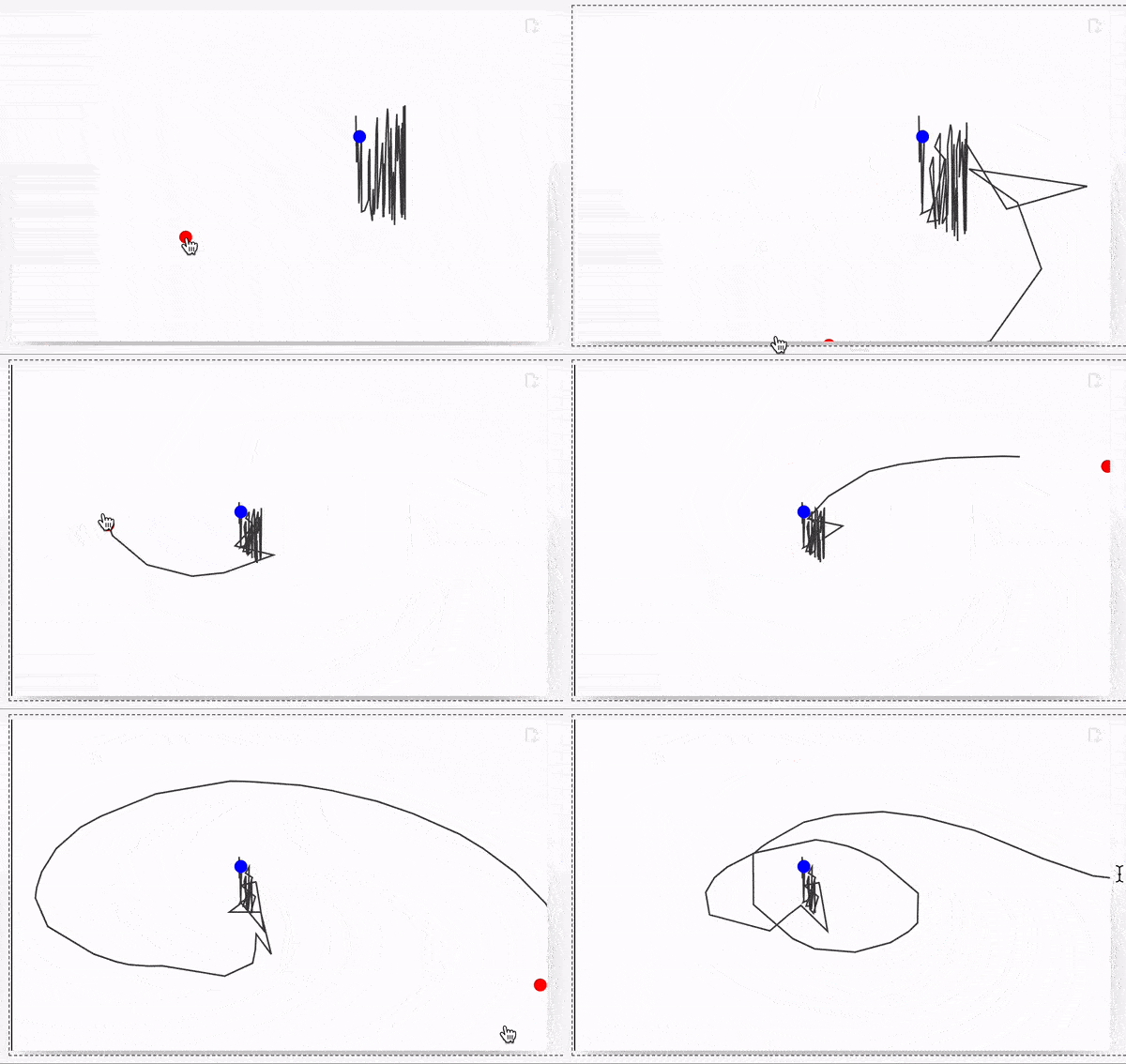
Try to drag a red dot using mouse The result will look like

Line interpolates missing segments of a line, if the dataset has been updated. No actions needed form the user